BIOKT Lab Handbook, Chapter 3: Checklist for MD Simulations¶

Status: v1 · Last revised: 2026-10-10

Source and licence. This chapter is an adaptation of the checklist and surrounding text in

E. Braun, J. Gilmer, H. B. Mayes, D. L. Mobley, J. I. Monroe, S. Prasad, D. M. Zuckerman, Best Practices for Foundations in Molecular Simulations [Article v1.0], Living J. Comp. Mol. Sci. 1, 5957 (2019). doi:10.33011/livecoms.1.1.5957

developed openly at github.com/MobleyLab/basic_simulation_training and released under the Creative Commons Attribution 4.0 International licence (CC BY 4.0). This chapter is distributed under the same licence.

What we changed. We reordered the material into the stages of a project, turned it into tick boxes, shortened the wording, and added material specific to how the BIOKT group works (GROMACS, intrinsically disordered proteins, validation between stages, record keeping). Items taken from the article are paraphrased, with a few short phrases kept from the original wording; §7 and the group-specific items are ours. Any errors introduced in the adaptation are ours, not the original authors'. Figures 1 and 2 are reproduced from the article; each caption states what we changed.

If you use this checklist in your own work, cite the original article, not this handbook.

1. Why this document exists¶

An MD simulation will almost always produce something: a trajectory, a movie, a number. Whether that something means anything depends on decisions made before the first step was integrated, many of which fail silently. The worst outcome is not a crash; it is a system that is not what you intended (wrong protonation state, missing ion, wrong water model) but is still chemically valid, so it runs cleanly through every subsequent step.

This checklist collects the decisions that matter and the checks that catch the most common mistakes. Go through it before you start a new project or a new set of systems, and again before you show results. It does not replace reading: for the concepts behind each item (ensembles, thermostats, long-range electrostatics, integrators), read the original article, which was written for exactly that purpose.

Keep the answers. Each decision below should be written down in your lab notebook or project README (Chapter 2, §7), with the reason, when you make it. "Why did you use this water model?" is a question you will be asked by a referee long after you have forgotten the answer.

2. Should you run MD at all?¶

MD is a tool, and it may not be the right one for your question. Before preparing anything:

Count the cost. What is the timescale of the process you want to observe? Is it tractable given the size of your system, the computing time available and the cost per ns? If the relevant events take milliseconds or longer, plain MD will not reach them.
Would the question be answered faster or more cheaply another way: an experiment, a collaborator, a simpler model?
If the feasibility is unclear, plan a small set of exploratory simulations to measure it, rather than plunging into the full study.
Have a rough idea of the statistical uncertainty you can expect, and whether it is small enough to answer the question (see §8).
For enhanced sampling (metadynamics, umbrella sampling, replica exchange), the same question applies to the chosen collective variables or replica ladder: is there a reason to think they capture the slow process?

3. Take stock of your plans¶

What question are you trying to answer, and what observable will answer it?
Which ensemble do you need (\(NVT\), \(NPT\), \(NVE\), \(\mu VT\))?
Which temperature, pressure and composition (salt concentration, pH, co-solvents)?
Which reference state or experiment are you trying to reproduce or predict?
Which force field properly describes your system?
What is already known in the literature, and which data will you compare to?
For intrinsically disordered proteins: force field and water model are a single choice. Combinations developed for folded proteins can produce disordered ensembles that are too compact. Check which combinations have been benchmarked for IDPs against data you can compare to (SAXS \(R_g\), NMR chemical shifts and \(J\)-couplings, FRET, PRE), and justify your choice in writing.
Decide now how many independent replicas you will run and from which starting structures (§6). This changes the cost estimate.

4. Prepare the system¶

A simulated box surrounded by its periodic images

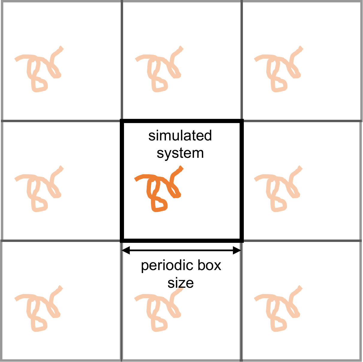
Figure 1. Periodic boundary conditions in two dimensions: the simulated system is surrounded by identical copies of itself. If the chain extends until it comes within a cutoff distance of its own image, it interacts with itself. Figure from Braun et al., LiveCoMS 1, 5957 (2019), CC BY 4.0; converted from PDF, caption rewritten.

Do not assume the system is correct because it runs. A badly prepared system often equilibrates without error. Inspect it visually and check its composition explicitly.

5. Choose simulation settings¶

5.1 Cutoffs and long-range interactions¶

Electrostatics are long-ranged: for periodic systems use a full treatment of long-range electrostatics (in practice PME). For finite systems the cutoff must exceed the system size.
Van der Waals interactions can usually be cut off at 1–1.5 nm, provided the box is at least twice the cutoff, but a long-range dispersion correction may be needed.
Use well-validated or default settings for the method, and deviate only after careful consideration and testing.
Cutoffs, switching or shifting functions and the dispersion correction are part of the force field. Use the settings with which the force field was parameterised (they differ between the Amber and CHARMM families), and cite where you took them from.

5.2 Thermostat, barostat and integrator¶

Choose a thermostat that gives the correct distribution of kinetic energies, not only the correct average. For small systems, or systems with weakly coupled components, choose one that works in the small-system limit.
Choose a barostat that gives the correct distribution of volumes.
Consider the known shortcomings of integrators, thermostats and barostats, and whether they affect the properties you will calculate (e.g. strong coupling to a stochastic thermostat slows dynamics, which matters for diffusion or kinetics).
In GROMACS terms: the Berendsen thermostat and barostat do not sample the correct ensemble and must not be used for production. v-rescale (thermostat) and C-rescale or Parrinello-Rahman (barostat) do. Parrinello-Rahman can oscillate badly far from equilibrium, so it is not suitable for the first steps of equilibration.

5.3 Timestep¶

Identify the highest-frequency motion in the system (usually bond vibrations involving hydrogen, unless those bonds are constrained).
As a first guess, set the timestep to about one tenth of the period of that motion.
Test the choice: in the microcanonical (\(NVE\)) ensemble, total energy should be conserved with no significant drift.
Standard practice with constrained bonds to hydrogen is 2 fs. A 4 fs timestep requires hydrogen mass repartitioning; if you use it, say so, and run the energy-conservation test above, because this is exactly the case the test is for.

6. Plan the run protocol¶

The standard sequence is: system preparation → energy minimisation → equilibration → production. The boundaries between these are not always sharp.

Plan how you will minimise and equilibrate, and test that your equilibration actually reaches equilibrium in the target ensemble. Typically: \(NVT\) to reach the target temperature, then \(NPT\) to reach the target density, before production in the target ensemble.
Never collect production data immediately after a change in conditions (box rescaling, minimisation, a jump in temperature or pressure).
Decide production length, and how often to save coordinates and energies. Saving far more often than the relevant correlation time fills disks with redundant data; saving energies and coordinates at commensurate intervals keeps structural and energetic analysis consistent.
Check that you have enough storage, memory and computer time for the whole plan, replicas included.
Independent replicas: different initial velocities give trajectories that diverge; different starting configurations give replicas that are independent from the outset, and are better.
Base the protocol on the group's established GROMACS workflow and .mdp templates rather than writing one from scratch. Any departure from it (new flag, new option, workaround) needs a reason written down.
Name stage outputs as described in Chapter 2, §3, from the first run.

6.1 A template script¶

If you have never set up a GROMACS simulation, work through a tutorial first: Justin Lemkul's Lysozyme in water or the official GROMACS tutorials. The script below follows the same steps as Lysozyme in water. It is not meant to be run as is. It shows how to write a setup script so that the choices made in §3–§5 appear once, at the top, and every file name is built from them:

model is the molecular model: system, force field and water model. The topology and starting structure depend only on these.
name is a simulation of that model under given conditions (here, temperature). Every output from NVT onwards carries it, plus the replica index.

Change the force field or temperature at the top, and every file name changes with it. Nothing is overwritten and you never type a file name by hand.

Each step is a few explicit lines, and the steps follow one another in the order you would type them. The script prints the checks of §7 as it goes (minimisation convergence, temperature, pressure, density), and stops if minimisation did not converge. The first time you use it on a new system, run it up to step 7 for one replica and look at the output before running production. A copy of the script and of ions.mdp (below) is in examples/gromacs/ of the project template.

#!/usr/bin/env bash
# scripts/run_md.sh: from a PDB file to production, one step after another.
# Run from the project root.
set -euo pipefail

# ---- What this run is. Only these lines change between runs. ---------------
sys=as4             # system identifier, fixed for the whole project
ff=amber99sb-ildn   # force field, as pdb2gmx names it (an example only: not for IDPs, §3)
fftag=a99sb         # short tag for the force field in file names
wat=tip3p           # water model
temp=300            # temperature (K)
conc=0.15           # NaCl concentration (mol/L), on top of neutralising ions
gmx=${GMX:-gmx}     # e.g. GMX=gmx_mpi where only the MPI build exists

# ---- Names, built from the choices above ----------------------------------
model=${sys}_${fftag}_${wat}    # e.g. as4_a99sb_tip3p
name=${model}_${temp}K          # e.g. as4_a99sb_tip3p_300K
top=setup/${model}.top
start=setup/${model}_start.gro  # solvated, neutralised starting structure
prep=data/prep/${model}
em=data/em/${model}_em
mkdir -p data/{prep,em,nvt,npt,md}

# ---- 1. Topology ----------------------------------------------------------
# Check protonation states (§4); -his lets you choose histidines.
# Run inside setup/ so that the topology includes its .itp files by name.
cd setup
$gmx pdb2gmx -f ${sys}.pdb -ff ${ff} -water ${wat} -ignh \
    -o ../${prep}_pdb2gmx.gro -p ${model}.top -i ${model}_posre.itp
cd ..

# ---- 2. Box ---------------------------------------------------------------
# 1.2 nm from solute to box edge. Not enough for an extended IDP (§4).
$gmx editconf -f ${prep}_pdb2gmx.gro -o ${prep}_box.gro -c -d 1.2 -bt dodecahedron

# ---- 3. Solvent -----------------------------------------------------------
# spc216.gro is the solvent box for 3-site water; use tip4p.gro for 4-site.
$gmx solvate -cp ${prep}_box.gro -cs spc216.gro -p ${top} -o ${prep}_solv.gro

# ---- 4. Ions --------------------------------------------------------------
$gmx grompp -f setup/mdp/ions.mdp -c ${prep}_solv.gro -p ${top} \
    -po ${prep}_ions_mdout.mdp -o ${prep}_ions.tpr
echo SOL | $gmx genion -s ${prep}_ions.tpr -p ${top} -o ${start} \
    -pname NA -nname CL -neutral -conc ${conc}

# ---- 5. Energy minimisation -----------------------------------------------
$gmx grompp -f setup/mdp/em.mdp -c ${start} -p ${top} -po ${em}_mdout.mdp -o ${em}.tpr
$gmx mdrun -deffnm ${em}
grep -E "converged to|Potential Energy|Maximum force" ${em}.log
grep -q "converged to Fmax" ${em}.log || { echo "EM did not converge" >&2; exit 1; }

# ---- 6-8. Equilibration and production, for each replica -------------------
# Replicas here differ only in their initial velocities (gen_seed = -1).
for rep in 0 1 2; do
  nvt=data/nvt/${name}_nvt_rep${rep}
  npt=data/npt/${name}_npt_rep${rep}
  md=data/md/${name}_md_rep${rep}

  # 6. NVT: bring the system to temperature, solute restrained
  sed "s/@TEMP@/${temp}/g" setup/mdp/nvt.mdp > ${nvt}.mdp
  $gmx grompp -f ${nvt}.mdp -c ${em}.gro -r ${em}.gro -p ${top} -po ${nvt}_mdout.mdp -o ${nvt}.tpr
  $gmx mdrun -deffnm ${nvt}
  echo Temperature | $gmx energy -f ${nvt}.edr -o ${nvt}_temperature.xvg

  # 7. NPT: bring the system to density, solute restrained
  sed "s/@TEMP@/${temp}/g" setup/mdp/npt.mdp > ${npt}.mdp
  $gmx grompp -f ${npt}.mdp -c ${nvt}.gro -r ${nvt}.gro -t ${nvt}.cpt -p ${top} \
      -po ${npt}_mdout.mdp -o ${npt}.tpr
  $gmx mdrun -deffnm ${npt}
  printf "Pressure\nDensity\n" | $gmx energy -f ${npt}.edr -o ${npt}_pressure_density.xvg

  # 8. Production
  sed "s/@TEMP@/${temp}/g" setup/mdp/md.mdp > ${md}.mdp
  $gmx grompp -f ${md}.mdp -c ${npt}.gro -t ${npt}.cpt -p ${top} -po ${md}_mdout.mdp -o ${md}.tpr
  $gmx mdrun -deffnm ${md}
done

The temperature enters the .mdp templates through a placeholder, e.g. in setup/mdp/nvt.mdp:

define    = -DPOSRES      ; restrain the solute while the solvent relaxes
tcoupl    = v-rescale
tc-grps   = System
tau_t     = 0.1
ref_t     = @TEMP@
gen_vel   = yes           ; new random velocities for each replica
gen_temp  = @TEMP@
gen_seed  = -1

The other settings in the templates (cutoffs, constraints, PME) come from the force field (§5.1) and stay fixed for the project.

One template is a special case. The .tpr built just before genion belongs to a system that is not yet neutral, and with PME grompp warns about the net charge, which stops the script. Do not reach for -maxwarn: that .tpr is only read by genion and never simulated, so give it plain cutoff electrostatics:

; setup/mdp/ions.mdp: only used to build the .tpr that genion reads
integrator    = steep
nsteps        = 50000
emtol         = 1000
cutoff-scheme = Verlet
coulombtype   = Cut-off   ; not PME: the system is not neutral yet
rcoulomb      = 1.0
rvdw          = 1.0

grompp then issues two notes, about the net charge and about the plain cutoff. Both are expected here, and neither applies to the simulation itself.

A few things the script deliberately leaves to you:

It stops on errors and on grompp warnings. set -e stops the script when a command fails, and grompp fails on any warning. Do not add -maxwarn to get past one (§7).
Replicas here differ only in their initial velocities. Starting them from different configurations is better (§6). To do that, give each replica its own starting structure and name it with rep<N>.
Production runs belong on the GPU servers or clusters. For real runs, move the production step (8) into a SLURM submission script in scripts/ rather than running it interactively.

7. Validate each stage before the next¶

This section goes beyond the original article, which describes what to look for during equilibration. We make it a rule that no stage starts until the previous one has been checked, because a mistake found three stages later costs far more than the check.

Every step: check the exit status, the end of the log file and that the expected output files exist. Do not chain stages in a script without these checks.
Warnings and notes are blockers. Every GROMACS (or Amber) note, warning or error must be understood and resolved. Never silence one with -maxwarn without writing down what it was and why it is safe.
Minimisation: converged (maximum force below the requested tolerance), with a negative and reasonable potential energy.
\(NVT\) equilibration: temperature fluctuates around the target with no drift.
\(NPT\) equilibration: pressure averages to the target (it fluctuates by hundreds of bar; judge the average) and density or box volume has stopped drifting.
Structural properties: the slow properties relevant to your question (RMSD, \(R_g\), secondary structure, contacts) show no systematic trend. For IDPs, RMSD to the starting structure says little; use \(R_g\), end-to-end distance or secondary-structure content.
If there is any ambiguity about whether a key property is still changing, extend equilibration.

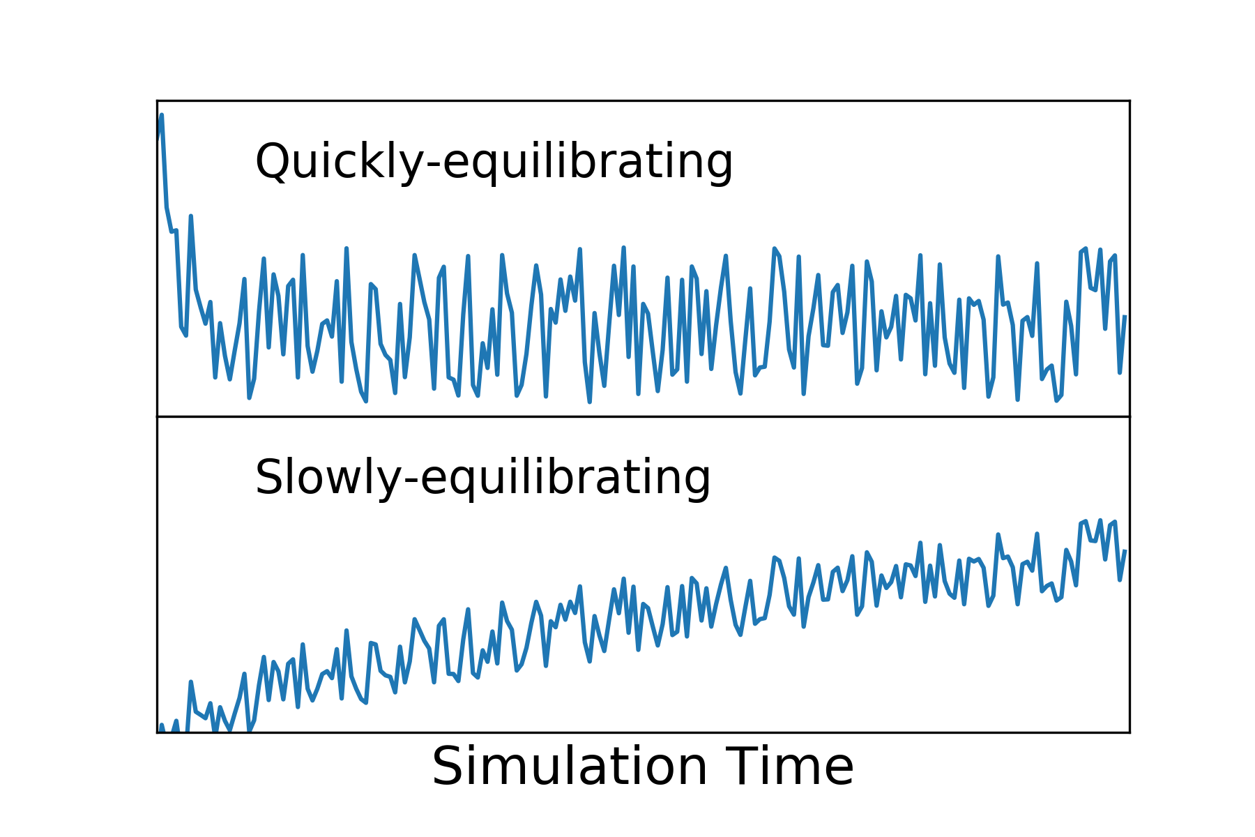
A quickly equilibrating property fluctuating around a constant value, and a slowly equilibrating one still drifting

Figure 2. Two properties of the same hypothetical simulation. The top one settles quickly and then fluctuates around a constant value; the bottom one is still drifting, so the system is not yet equilibrated. Temperature and pressure usually behave like the top panel; slow structural properties often behave like the bottom one. Figure from Braun et al., LiveCoMS 1, 5957 (2019), CC BY 4.0; background made opaque, caption rewritten. - [ ] Record the key numbers (average \(T\), \(P\), density, energies) in your lab notebook, so that you can compare across systems and replicas.

8. Use the results with care¶

Treat an MD result as the outcome of a computational experiment with a particular model, composition and protocol, not as "the answer".
Do not over-interpret short or unequilibrated simulations. A movie is not a result.
When comparing systems (wild type vs mutant, two conditions), remember that replicas of the same system diverge. A difference between two single trajectories may be noise; you need replicas or error bars to tell.
Every reported average needs an uncertainty estimate that accounts for time correlation (e.g. block averaging). See the companion article: A. Grossfield et al., Best Practices for Quantification of Uncertainty and Sampling Quality in Molecular Simulations [Article v1.0], Living J. Comp. Mol. Sci. 1, 5067 (2019), doi:10.33011/livecoms.1.1.5067.
Check convergence: does the estimate change if you use only the first or second half of the production data, or drop one replica?
Compare with experiment where data exist, and report disagreement as well as agreement.

9. Further reading¶

The original article (§ Source above) explains every concept this checklist relies on and points to textbooks and tutorials for each.
Justin Lemkul's GROMACS tutorials, mdtutorials.com, are the usual starting point for hands-on practice. The official GROMACS tutorials cover more advanced topics (free energies, umbrella sampling) as interactive notebooks.
Chapter 2 of this handbook, for where all of the above is recorded.

BIOKT Lab Handbook, BIOKT group (UPV/EHU – DIPC). Chapter 3. Adapted from Braun et al., LiveCoMS 1, 5957 (2019), CC BY 4.0.